IISPH — Reproduction Notes (Paper)
Paper: Markus Ihmsen, Jens Cornelis, Barbara Solenthaler, Christopher Horvath, Matthias Teschner. Implicit Incompressible SPH. IEEE Transactions on Visualization and Computer Graphics, July 2013. DOI: 10.1109/TVCG.2013.105
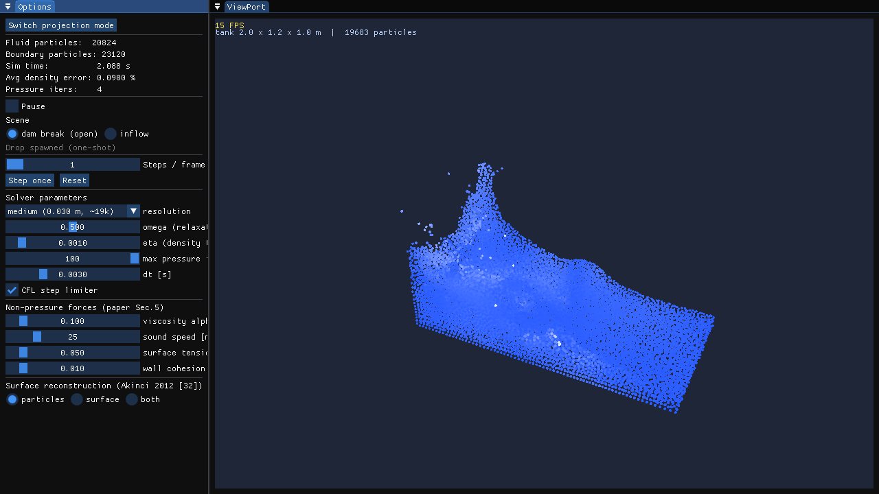
headless, 1920x1080, 120fps, 64000 particles, grid 0.5, DFSPH
Prerequisite Knowledge
Dirac delta function
The Dirac delta $\delta(x)$ is the “point mass” distribution characterized by its sifting property: for any continuous function $f$,
$$ \int_{-\infty}^{+\infty} f(x)\, \delta(x - a)\, dx = f(a). $$Intuitively: $\delta(x-a)$ is infinitely tall, infinitely thin, sits at $x=a$, and has integral $1$. It is the mathematical tool that says “all the mass of a point particle is concentrated at one location”.
Point-particle density and the idea of SPH
A set of point particles with masses $m_j$ at positions $x_j$ has the exact density field
$$ \rho(x) = \sum_j m_j\, \delta(x - x_j). $$Check: integrate over all space,
$$ \int \rho(x)\, dx = \sum_j m_j \int \delta(x-x_j)\, dx = \sum_j m_j, $$which is exactly the total mass. Good. Problem: $\delta$ is useless numerically — the density is $0$ almost everywhere and infinite at the particles; we cannot differentiate or sample it. Idea of SPH (Smoothed Particle Hydrodynamics): replace $\delta$ by a smooth function $W_h$ that approximates it:
$$ \delta(x) \;\approx\; W_h(x), \qquad W_h \to \delta \text{ as } h \to 0. $$$W_h$ is called the kernel function (or smoothing kernel); $h$ is its support radius (also called smoothing length). Then the density at particle $i$ is approximated by sampling the smoothed field at $x_i$:
$$ \rho_i = \sum_j m_j\, W_{ij}, \qquad W_{ij} := W(x_i - x_j). \tag{paper Sec.2} $$Why this is a valid density: because $\int W = 1$ (normalization), the total mass is still $\sum_j m_j$, and $\rho_i$ is large where particles are crowded — exactly the behavior of a real density.
Requirements on the kernel $W$
- Normalization: $\int W(x), dx = 1$ — total mass preserved.
- Finite support: $W(x) = 0$ for $|x| > h$ — each particle only interacts with neighbors inside radius $h$; cost stays $O(\text{neighbors})$.
- Smoothness: $W$ differentiable (we need $\nabla W$ for pressure forces).
- Radial symmetry / decay: $W$ depends on $|x|$ and decreases with distance.
- $W’(0) = 0$ (i.e. $\nabla W = 0$ at the origin) — the cubic spline kernel used in the paper satisfies this; it makes the self-interaction term vanish automatically.
The general SPH interpolation formula
Any field $A(x)$ can be reconstructed from its values at the particles. Start from the exact reconstruction (sifting property again),
$$ A(x) = \int A(x')\, \delta(x - x')\, dx'. $$Replace $\delta$ by $W$, replace the integral by a sum over particles, and identify the volume element of particle $j$ with its physical volume $V_j = m_j / \rho_j$ (mass over density — mass conservation per particle):
$$ A(x) \approx \sum_j A_j\, \frac{m_j}{\rho_j}\, W(x - x_j). $$Sampled at particle $i$:
$$ A_i \approx \sum_j m_j \frac{A_j}{\rho_j}\, W_{ij}. \tag{SPH interpolation} $$If $A = \rho$, then $A_j/\rho_j = 1$ and we recover the density formula above — so the density formula is just the special case $A = \rho$ of the interpolation formula. Differentiating the interpolation formula: $A_j, \rho_j$ are constants attached to particle $j$; only $W$ depends on position. Hence
$$ \nabla A(x_i) \approx \sum_j m_j \frac{A_j}{\rho_j}\, \nabla W_{ij}. \tag{SPH gradient} $$Vector calculus basics (from the Stable Fluids notes, restated)
- Gradient $\nabla f = (\partial f/\partial x, \partial f/\partial y, \partial f/\partial z)$: the steepest-ascent direction of a scalar field.
- Divergence $\nabla\cdot u = \partial u/\partial x + \partial v/\partial y + \partial w/\partial z$: local rate of volume expansion of a vector field.
- Laplacian $\nabla^2 f = \nabla\cdot(\nabla f)$: divergence of the gradient.
- Product rule (vector form): $\nabla\cdot(f u) = f,\nabla\cdot u + u\cdot\nabla f$.
- Scalar triple product: $a\cdot(b\times c) = b\cdot(c\times a) = c\cdot(a\times b)$.
Material derivative
$$ \frac{D}{Dt} = \frac{\partial}{\partial t} + v\cdot\nabla $$is the rate of change seen by an observer moving with the fluid. SPH particles are fluid parcels, so the rate of change of a quantity attached to particle $i$ is a material derivative — which is why we may discretize time derivatives on particles with plain finite differences.
Euler time integration
- Forward (explicit) Euler: $f^{n+1} = f^n + \Delta t, g(f^n)$ — simple but restricted by a stability condition on $\Delta t$.
- Backward (implicit) Euler: $f^{n+1} = f^n + \Delta t, g(f^{n+1})$ — unconditionally stable for the model problem $\dot f = -a f$, but requires solving an equation.
- Semi-implicit Euler: some terms use $t$ (explicit), others $t+\Delta t$ (implicit). IISPH uses this: velocities are implicit through the unknown pressure forces, while the kernel gradients are evaluated at the known time $t$.
Artificial viscosity (Monaghan 1992/2005, cited as [23] in the paper)
Real fluids have viscosity: neighboring fluid elements resist relative motion. In SPH this shows up as a force proportional to the velocity gradient. The paper’s framework uses the artificial viscosity of Monaghan (the classic SPH viscosity, present in both the 1992 and the 2005 survey; the paper cites the 2005 one as [23]).
The idea
Consider a pair of particles $i, j$ with relative velocity $\mathbf{v}_{ij} = \mathbf{v}_{i} - \mathbf{v}_{j}$ and relative position $\mathbf{r}_{ij} = \mathbf{x}_{i} - \mathbf{x}_{j}$.
If $\mathbf{v}_{ij} \cdot \mathbf{r}_{ij} < 0$ , the particles are approaching each other;
If $\mathbf{v}_{ij} \cdot \mathbf{r}_{ij} > 0 $ they are separating. Viscosity should damp the approaching motion (it resists compression of the flow) and leave separating motion alone. Monaghan’s artificial viscosity adds, for approaching pairs, an extra “pressure-like” term:
$$ \Pi_{ij} = -\alpha, \bar{c}_{ij}, \frac{\mu_{ij}}{\bar\rho_{ij}}, \qquad \mu_{ij} = \frac{h, \mathbf{v}_{ij}\cdot\mathbf{r}_{ij}}{|\mathbf{r}_{ij}|^2 + 0.01 h^2}, \qquad (\text{if } \mathbf{v}_{ij}\cdot\mathbf{r}_{ij} < 0) $$- $\Pi_{ij} = 0$ when $\mathbf{v}_{ij}\cdot\mathbf{r}_{ij} \ge 0$ (separating pairs).
- $\alpha$: dimensionless strength (paper-scale values $\sim 0.01$–$0.1$; SPlisHSPlasH’s implementation calls this model Monaghan1992).
- $\bar c_{ij}$: average artificial speed of sound — a numerical parameter that sets the compressibility scale of the flow.
- $\bar\rho_{ij} = (\rho_i + \rho_j)/2$: average density.
- The term $0.01 h^2$ in the denominator only prevents division by zero when two particles are on top of each other. Since $\mu_{ij} < 0$ for approaching pairs, $\Pi_{ij} > 0$: it acts like a small repulsive pressure that slows the approach — a cheap numerical viscosity.
The force
The viscosity acceleration is the SPH-weighted sum of $\Pi$ over the kernel gradient (derivation: it is a momentum-preserving anti-symmetric pairwise force, exactly like the pressure force (2) with $p_i/\rho_i^2 \to \Pi_{ij}/2$-style symmetrization):
$$ \mathbf{a}^{\text{visc}}_i = \sum_j m_j\, \Pi_{ij}\, \nabla_{\!i} W_{ij}, \qquad \Pi_{ij} = \Pi_{ji} \ \text{(anti-symmetric force pair)}. $$In our normalized form ($\rho_n = \rho/\rho_0$, $V = $ particle volume, so $m_j/\bar\rho_{ij} = V_j/\bar\rho_{n,ij}$):
$$ \mathbf{a}^{\text{visc}}_i = -\sum_j V_j\, \frac{\alpha c\, \mu_{ij}}{\bar\rho_{n,ij}}\, \nabla_{\!i} W_{ij} $$with the minus sign because $\mu_{ij} < 0$ (the code evaluates $\Pi_{ij}$ and accumulates $\mathbf{a} -= V_j \Pi_{ij} \nabla W$). It is evaluated in the advection phase (a non-pressure force), i.e. it contributes to $\mathbf{v}^{\text{adv}}$.
Linear systems and (relaxed) Jacobi iteration
A linear system $A p = b$ ($A$ an $n\times n$ matrix, $p, b$ vectors) can be solved by splitting $A = D + R$ where $D$ is the diagonal part of $A$. The equation for row $i$,
$$ a_{ii}\, p_i = b_i - \sum_{j\neq i} a_{ij}\, p_j, $$suggests the Jacobi iteration (all unknowns updated simultaneously using the previous iterate):
$$ p^{l+1}_i = \frac{1}{a_{ii}}\left(b_i - \sum_{j\neq i} a_{ij} p^l_j\right), \qquad l = 0, 1, 2, \dots $$Relaxed (weighted) Jacobi mixes the new value with the old one using a relaxation factor $\omega$:
$$ p^{l+1}_i = (1-\omega)\, p^l_i + \omega\, \frac{1}{a_{ii}}\left(b_i - \sum_{j\neq i} a_{ij} p^l_j\right). $$- $\omega = 1$: plain Jacobi.
- $0 < \omega < 1$: damping — suppresses the oscillation that plain Jacobi suffers from on smooth error components. The paper uses $\omega = 0.5$. Jacobi requires no special structure of $A$ (no symmetry needed), which matters here because the IISPH system matrix is not symmetric (see Sec. 3.2 of the paper).
Paper
The problem: enforcing incompressibility in SPH
Water is nearly incompressible: its density barely changes. In SPH, “incompressible” means “keep $\rho_i \approx \rho_0$ for every particle $i$” ($\rho_0$ = rest density). The paper’s goal: an implicit projection method for SPH that (a) converges fast, (b) allows large time steps, (c) scales to millions of particles. Roadmap of the method (one time step):
| |
This is the classical projection / splitting idea: predict with the known parts, then project onto the constraint (here: density = rho_0) using the unknown pressure.
Standard SPH ingredients used by the paper
Density (already derived in Prerequisite §2)
$$ \rho_i(t) = \sum_j m_j\, W_{ij}(t), \qquad W_{ij}(t) = W(x_i(t) - x_j(t)). \tag{paper Sec.2} $$Equation of state (EOS) — the “old” way to get pressure
$$ p_i(t) = \frac{\kappa \rho_0}{\gamma}\left[\left(\frac{\rho_i(t)}{\rho_0}\right)^\gamma - 1\right]. \tag{1} $$- $\rho_0$: rest density (e.g. 1000 kg/m³ for water).
- $\kappa$: stiffness (user parameter).
- $\gamma$: exponent, typically 7. With $\gamma = 7$, a small density increase produces an enormous pressure — water “fights back” against compression. This is an equation of state: it relates the thermodynamic state variables (here: density) to the pressure. Standard/weakly compressible SPH (SSPH/WCSPH) computes $p$ from (1) directly. IISPH does NOT use (1); it solves a linear system so that $\rho_i(t+\Delta t) = \rho_0$ exactly (implicitly). (1) is included for context.
The symmetric pressure force (Eqn. 2) — full derivation
We want the force on particle $i$ due to pressure. In the continuum, the pressure force per unit volume is $-\nabla p$ (pressure pushes from high to low). Particle $i$ occupies volume $V_i = m_i/\rho_i$, so:
$$F^p_i = V_i\,(-\nabla p)(x_i) = -\frac{m_i}{\rho_i}\,\nabla p(x_i). \tag{A}$$
Step 1 — naive discretization, and why it fails. Using the SPH gradient formula with $A = p$:
$$ \nabla p(x_i) \approx \sum_j m_j \frac{p_j}{\rho_j}\, \nabla W_{ij}, \qquad\text{so}\qquad F^p_i = -\frac{m_i}{\rho_i}\sum_j m_j \frac{p_j}{\rho_j}\, \nabla W_{ij}. \tag{B} $$$F^P_i$ is the forces that particle $i$ receives from all the neighbor particles $j$. We can look at the force of particle $j$ to particle $i$ individually by take a certain term in the sum. The force that particle $j$ receives from $i$ is obtained by swapping $i\leftrightarrow j$ and using $\nabla W_{ji} = -\nabla W_{ij}$ (gradient is anti-symmetric in the pair):
$$ F^p_{j\leftarrow i} = -\frac{m_j}{\rho_j} m_i \frac{p_i}{\rho_i}\, \nabla W_{ji} = + \frac{m_i m_j}{\rho_i\rho_j}\, p_i\, \nabla W_{ij}, \qquad F^p_{i\leftarrow j} = -\frac{m_i m_j}{\rho_i\rho_j}\, p_j\, \nabla W_{ij}. $$These are not equal and opposite ($p_i \neq p_j$ in general) — Newton’s third law is violated, momentum is not conserved, and the fluid would drift. We need a symmetric discretization. Step 2 — a calculus identity. Start from the product rule for the gradient of a quotient $p/\rho$:
$$ \nabla\left(\frac{p}{\rho}\right) = \frac{1}{\rho}\nabla p + p\,\nabla\left(\frac{1}{\rho}\right), \qquad \nabla\left(\frac{1}{\rho}\right) = -\frac{1}{\rho^2}\nabla\rho . $$Therefore
$$ \nabla\left(\frac{p}{\rho}\right) = \frac{1}{\rho}\nabla p - \frac{p}{\rho^2}\nabla\rho, \qquad\text{i.e.}\qquad \boxed{\;\frac{\nabla p}{\rho} = \nabla\left(\frac{p}{\rho}\right) + \frac{p}{\rho^2}\nabla\rho\;} \tag{C} $$Step 3 — discretize the two terms of (C) at $x_i$.
- First term $\nabla(p/\rho)$: use SPH gradient with $A = p/\rho$: $$ \nabla\left(\frac{p}{\rho}\right)\bigg|_{x_i} = \sum_j m_j\, \frac{p_j/\rho_j}{\rho_j}\, \nabla W_{ij} = \sum_j m_j \frac{p_j}{\rho_j^2}\, \nabla W_{ij}. $$
- Second term $\frac{p_i}{\rho_i^2}\nabla\rho$: use the density gradient $\nabla\rho(x_i) = \sum_j m_j \nabla W_{ij}$: $$ \frac{p_i}{\rho_i^2}\, \nabla\rho(x_i) = \frac{p_i}{\rho_i^2}\sum_j m_j \nabla W_{ij} = \sum_j m_j \frac{p_i}{\rho_i^2}\, \nabla W_{ij}. $$ Step 4 — combine. Both terms are sums over $j$ of $m_j\nabla W_{ij}$; factor them:
Multiply by $-m_i$ (from (A)):
$$ \boxed{\;F^p_i(t) = -m_i \sum_j m_j \left(\frac{p_i(t)}{\rho_i^2(t)} + \frac{p_j(t)}{\rho_j^2(t)}\right)\nabla W_{ij}(t)\;} \tag{2} $$Step 5 — verify momentum conservation. Swap $i \leftrightarrow j$: the bracket $p_i/\rho_i^2 + p_j/\rho_j^2$ is invariant, $\nabla W_{ji} = -\nabla W_{ij}$, so $F^p_{j\leftarrow i} = -F^p_{i\leftarrow j}$. Newton’s third law holds. This symmetric form is the reason the paper uses it (it is attributed to [1] = Gingold & Monaghan). Physical notes: on the free surface a particle has no neighbors on the outside, so the sum only contains interior neighbors with positive pressure, pushing it inward — the atmosphere pushing on the surface, automatic. And if $p = 0$ everywhere, $F^p = 0$ — no spurious forces.
The IISPH derivation (paper Sec. 2.1)
The continuity equation
Conservation of mass for a fluid parcel of density $\rho$ and volume $V$: $m = \rho V$ is constant, so its material derivative vanishes:
$$ \frac{D(\rho V)}{Dt} = V\frac{D\rho}{Dt} + \rho\frac{DV}{Dt} = 0 \quad\Longrightarrow\quad \frac{D\rho}{Dt} = -\rho\,\frac{1}{V}\frac{DV}{Dt}. $$The relative rate of volume change of a parcel equals the divergence of the velocity field, $\frac{1}{V}\frac{DV}{Dt} = \nabla\cdot v$ (divergence = local expansion rate). Hence the continuity equation:
$$ \frac{D\rho}{Dt} = -\rho\, \nabla\cdot v. \tag{continuity} $$Meaning: $\nabla\cdot v > 0$ (particles moving apart) lowers the density; $\nabla\cdot v < 0$ raises it.
SPH discretization of the divergence
We need $\nabla\cdot v$ at particle $i$ in terms of kernel functions. Use the vector product rule with $f = \rho$:
$$ \nabla\cdot(\rho v) = \rho\,\nabla\cdot v + v\cdot\nabla\rho \quad\Longrightarrow\quad \nabla\cdot v = \frac{1}{\rho}\left(\nabla\cdot(\rho v) - v\cdot\nabla\rho\right). $$Discretize both terms at $x_i$ with SPH interpolation ($A = \rho v$ for the first, $A=\rho$ for the second):
$$ \nabla\cdot(\rho v)(x_i) \approx \sum_j m_j\, v_j\cdot\nabla W_{ij}, \qquad \nabla\rho(x_i) \approx \sum_j m_j\, \nabla W_{ij}. $$(The gradient acts only on $W$; particle values $v_j, \rho_j$ are constants.) Substitute and collect:
$$ \nabla\cdot v_i = \frac{1}{\rho_i}\left(\sum_j m_j\, v_j\cdot\nabla W_{ij} - v_i\cdot\sum_j m_j\nabla W_{ij}\right) = \frac{1}{\rho_i}\sum_j m_j\,(v_j - v_i)\cdot\nabla W_{ij}. $$With the relative velocity $v_{ij} := v_i - v_j$, we have $v_j - v_i = -v_{ij}$, so:
$$ \boxed{\;\nabla\cdot v_i = -\frac{1}{\rho_i}\sum_j m_j\, v_{ij}\cdot\nabla W_{ij}\;} \tag{paper Sec.2.1} $$Discretize the continuity equation (paper Eqn. 3)
Plug the SPH divergence into the continuity equation at particle $i$:
$$ \frac{D\rho_i}{Dt} = -\rho_i\, \nabla\cdot v_i = -\rho_i \left(-\frac{1}{\rho_i}\sum_j m_j v_{ij}\cdot\nabla W_{ij}\right) = \sum_j m_j\, v_{ij}\cdot\nabla W_{ij}. $$Now discretize the time derivative with a forward difference on the particle, and evaluate the right-hand side at the future time $t+\Delta t$ (this is where the implicitness comes from):
$$ \frac{\rho_i(t+\Delta t) - \rho_i(t)}{\Delta t} = \sum_j m_j\, v_{ij}(t+\Delta t)\cdot\nabla W_{ij}(t). \tag{3} $$Note: the kernel gradient is evaluated at time $t$ (known), while the velocities are at $t+\Delta t$ (unknown). Using the known $\nabla W_{ij}(t)$ instead of $\nabla W_{ij}(t+\Delta t)$ introduces only an $O(\Delta t)$ error (same order as the rest of the discretization) but avoids recomputing the neighborhood — the paper’s “velocity-based” source term (Sec. 2.2).
Semi-implicit Euler split of the velocity
Newton’s law per particle: $m_i \dot v_i = F^{adv}_i + F^p_i$, where $F^{adv}$ collects all known non-pressure forces (gravity, viscosity, surface tension). A semi-implicit Euler step:
$$ v_i(t+\Delta t) = v_i(t) + \Delta t\, \frac{F^{adv}_i(t) + F^p_i(t)}{m_i}. $$Prediction (projection’s predict step): drop the pressure forces and define the intermediate (advected) velocity
$$ v^{adv}_i = v_i(t) + \Delta t\, \frac{F^{adv}_i(t)}{m_i}. \tag{4a} $$Then the future velocity is $v_i(t+\Delta t) = v^{adv}_i + \Delta t, F^p_i(t)/m_i$. Predicted density: plug the predicted velocities into (3) (with $\rho_i(t+\Delta t)$ replaced by the predicted value):
$$ \rho^{adv}_i = \rho_i(t) + \Delta t \sum_j m_j\, v^{adv}_{ij}\cdot\nabla W_{ij}(t). \tag{4} $$Everything on the right is known. $\rho^{adv}_i$ is the density that the particles would have after one step if no pressure acted.
The pressure equation (paper Eqn. 5)
We now demand: after the full step, the density is exactly the rest density, $\rho_i(t+\Delta t) = \rho_0$ (density invariance condition). Write (3) for the full step using $v(t+\Delta t) = v^{adv} + \Delta t F^p/m$:
$$ \rho_i(t+\Delta t) = \rho_i(t) + \Delta t \sum_j m_j \left(v^{adv}_{ij} + \Delta t\left(\frac{F^p_i}{m_i} - \frac{F^p_j}{m_j}\right)\right)\cdot\nabla W_{ij}. $$Split the sum: the $v^{adv}$ part is exactly $\rho^{adv}_i - \rho_i(t)$ by (4). Setting $\rho_i(t+\Delta t) = \rho_0$:
$$ \rho_0 = \rho^{adv}_i + \Delta t^2 \sum_j m_j \left(\frac{F^p_i}{m_i} - \frac{F^p_j}{m_j}\right)\cdot\nabla W_{ij}, $$i.e.
$$ \boxed{\;\Delta t^2 \sum_j m_j \left(\frac{F^p_i}{m_i} - \frac{F^p_j}{m_j}\right)\cdot\nabla W_{ij} = \rho_0 - \rho^{adv}_i\;} \tag{5} $$Interpretation: the left side is “the density change caused by the pressure forces”; the right side is “the density deficit that must be repaired”. This is the discrete pressure Poisson equation (PPE) of the method.
The linear system (paper Eqn. 6)
$F^p$ depends linearly on the unknown pressures $p_j$ through (2). Substituting (2) into (5), each equation becomes
$$ \sum_j a_{ij}\, p_j = b_i, \qquad b_i := \rho_0 - \rho^{adv}_i. \tag{6} $$One equation and one unknown pressure per particle: $A p = b$ with the “source term” $b_i = \rho_0 - \rho^{adv}_i$. Remark (paper Sec. 2.2): the paper prefers this density source term over the divergence source term $\nabla\cdot v^{adv}$ used by some ISPH variants, because a divergence constraint accumulates unperceived volume loss over time in Lagrangian methods, whereas a density constraint directly monitors volume.
Solving the system: relaxed Jacobi (paper Sec. 3.1)
We never form the matrix $A$ explicitly (“matrix-free”). We need two ingredients for the Jacobi update of row $i$: the diagonal $a_{ii}$, and the off-diagonal action $\sum_{j\neq i} a_{ij} p^l_j$.
Extracting the coefficients: the displacement of (9)
Substitute the pressure force (2) into the pressure-induced displacement $\Delta t^2 F^p_i/m_i$ and separate the term proportional to $p_i$ from the terms proportional to the neighbors’ pressures $p_j$:
$$ \begin{aligned} \Delta t^2 \frac{F^p\_i}{m\_i} &= -\Delta t^2 \sum\_j m\_j \left(\frac{p\_i}{\rho\_i^2} + \frac{p\_j}{\rho\_j^2}\right)\nabla W\_{ij} \\ &= \underbrace{\left(-\Delta t^2 \sum\_j \frac{m\_j}{\rho\_i^2}\nabla W\_{ij}\right)}_{=:\, d\_{ii}} p\_i + \sum\_j \underbrace{\left(-\Delta t^2 \frac{m\_j}{\rho\_j^2}\nabla W\_{ij}\right)}_{=:\, d\_{ij}} p\_j . \end{aligned} \tag{9} $$IMPORTANT — these $d$’s are vectors ($\nabla W_{ij}$ is a vector). The “product” $d_{ii} p_i$ is a scalar-times-vector; when a $d$ appears inside a sum multiplied by $m_j\nabla W_{ij}$ later, the pairing is a dot product. Meaning: $d_{ii} p_i$ = the displacement of particle $i$ caused by its own pressure; $d_{ij} p_j$ = the displacement caused by neighbor $j$’s pressure.
Assembling $a_{ii}$ (paper Eqns. 10–12)
Plug (9) into (5). The displacement difference in (5) is
$$ \Delta t^2\left(\frac{F^p_i}{m_i} - \frac{F^p_j}{m_j}\right) = \left(d_{ii} p_i + \sum_j d_{ij} p_j\right) - \left(d_{jj} p_j + \sum_k d_{jk} p_k\right), $$where $j$ runs over the neighbors of $i$, and $k$ over the neighbors of $j$ — note the neighbors of the neighbors appear (second ring). Equation (5) becomes
$$ \rho_0 - \rho^{adv}_i = \sum_j m_j \left( d_{ii} p_i + \sum_j d_{ij} p_j - d_{jj} p_j - \sum_k d_{jk} p_k \right)\cdot\nabla W_{ij}. \tag{10} $$(Here and below the inner sum $\sum_j d_{ij} p_j$ runs over the same neighbor set as the outer sum; to avoid confusion we will write it as $\sum_{j’} d_{ij’} p_{j’}$ when needed.) Separate $p_i$. The value $p_i$ appears in two places:
- The explicit $d_{ii} p_i$ term.
- Inside $\sum_k d_{jk} p_k$ when $k = i$ — this is $d_{ji} p_i$. Split the $k$-sum accordingly:
(There is no $p_i$ inside $\sum_{j’} d_{ij’} p_{j’}$ because $j’ = i$ would give $d_{ii} p_i = -\Delta t^2 (m_i/\rho_i^2)\nabla W_{ii} p_i = 0$ — the kernel gradient at the origin vanishes, requirement 5 of Prerequisite §3.) Collecting all terms proportional to $p_i$ in (10): from the first part, $\sum_j m_j, d_{ii}\cdot\nabla W_{ij}, p_i$ (note $d_{ii}$ does not depend on the outer index $j$), and from (11), $-\sum_j m_j, d_{ji}\cdot\nabla W_{ij}, p_i$. Hence the diagonal coefficient is
$$ \boxed{\;a_{ii} = \sum_j m_j\, (d_{ii} - d_{ji})\cdot\nabla W_{ij}\;} \tag{12} $$a scalar (dot products), as required for the Jacobi denominator.
The relaxed Jacobi update (paper Eqns. 8 and 13)
The generic relaxed Jacobi formula for (6) is (8):
$$ p^{l+1}_i = (1-\omega)\, p^l_i + \omega\, \frac{1}{a_{ii}}\left(\rho_0 - \rho^{adv}_i - \sum_{j\neq i} a_{ij} p^l_j\right). \tag{8} $$Instead of computing $a_{ij}$ explicitly, we use the $d$-form of the off-diagonal action from (10), keeping only the parts that do not contain $p_i$ (those parts went into $a_{ii}$). The result is the paper’s Eqn. 13:
$$ p^{l+1}_i = (1-\omega)\, p^l_i + \frac{\omega}{a_{ii}}\left[\rho_0 - \rho^{adv}_i - \sum_j m_j \left( \sum_{j'} d_{ij'} p^l_{j'} - d_{jj} p^l_j - \sum_{k\neq i} d_{jk} p^l_k \right)\cdot\nabla W_{ij} \right]. \tag{13} $$Efficient implementation (paper Sec. 3.1.1)
Two passes per iteration, both over all particles, no data dependencies between them (parallel-friendly):
Pass 1: compute and store, per particle $i$, $S_i := \sum_{j} d_{ij} p^l_j = \Delta t^2 \sum_j \left(-\frac{m_j}{\rho_j^2}\nabla W_{ij}\right) p^l_j$.
Pass 2: for each particle $i$, compute $p^{l+1}_i$ with (13). The term $\sum_{k\neq i} d_{jk} p^l_k$ is obtained from the stored value at neighbor $j$ as $S_j - d_{ji} p^l_i$. Storage per particle: only $a_{ii}$, $d_{ii}$, $S_i$, $\rho_i$, $\rho^{adv}_i$, $p_i$ and $v^{adv}_i$ — the paper says “seven scalar values per particle” (plus the density/velocity fields themselves). $d_{ij}$ and $a_{ij}$ are never stored. Convergence parameters (paper observations):
Relaxation factor $\omega = 0.5$ is optimal across all their settings.
Initial pressure $p^0_i = 0.5, p_i(t-\Delta t)$ (warm start from the previous step; plain $p_i(t-\Delta t)$ or $0$ converge slower).
Convergence criterion: average density error $\eta = 0.1%$ recommended (max-error of 1% causes surface oscillations; average error controls global volume change).
At least 2 iterations regardless ($l < 2$ guard in Algorithm 1).
Negative pressure clamping: pressures can come out negative when $\rho^{adv}_i < \rho_0$, producing attracting pressure forces — exaggerated “surface tension” that swallows splashes (paper Fig. 2). EOS solvers avoid this by clamping negative pressures to zero; IISPH does the same, clamping $p_i \ge 0$ each iteration. (This is only safe with Jacobi; see §4.5.)
Why not Conjugate Gradient (paper Sec. 3.2)
The paper implemented CG with diagonal preconditioning but reports two problems:
- Non-symmetry. $a_{ij}$ is scaled by $m_i/\rho_i^2$, so $a_{ij} \neq a_{ji}$. CG requires a symmetric positive-definite matrix. One could force symmetry by assuming $\rho_i = \rho_j = \rho_0$, $m_i = m_j$ — valid for uniform sampling but wrong for adaptive or multi-phase SPH. Relaxed Jacobi does not care about symmetry.
- Negative-pressure clamping. Clamping between CG iterations destroys the conjugate-gradient recurrence (the system changes mid-solve) and causes instabilities. Jacobi tolerates clamping because each update only uses the current values. Conclusion of the paper: for this system, relaxed Jacobi is the practical choice.
Boundary handling (paper Sec. 4)
The problem and the chosen scheme
Fluid particles near a solid boundary have no neighbors on the solid side, so nothing stops them from penetrating the wall. IISPH is agnostic about boundary handling; the paper pairs it with the rigid-fluid coupling of [29] (Akinci et al. 2012): a layer of boundary particles $b$ is placed on the solid surface. They contribute to the density and forces of fluid particles but do not move and carry no pressure of their own.
Normalizing the boundary contribution: $\Psi^b$
Boundary particles are not fluid; giving them a raw mass would mis-calibrate the density near walls. The scheme normalizes by the number density of the boundary at the fluid particle:
$$ \delta^b_i \equiv \sum_{b} W^b_{ib}, \qquad \Psi^b(\rho^0_i) = \frac{\rho^0_i}{\delta^b_i}. $$- $\delta^b_i$ = sum of boundary kernel values at $x_i$ — “how densely the wall is packed” in kernel units.
- $\Psi^b$ = the equivalent fluid density contributed by one boundary particle, chosen so that the boundary contributes to $\rho_i$ on the same scale as fluid neighbors.
Density estimation with boundaries (paper Eqn. 14)
Every fluid term gets a boundary counterpart:
$$ \begin{align} \rho_i(t+\Delta t) =& \underbrace{\sum_j m_j W_{ij}}_{\text{fluid static}} + \underbrace{\sum_b \Psi^b(\rho^0_i) W^b_{ib}}_{\text{boundary static}} + \Delta t \sum_j m_j v_{ij}(t+\Delta t)\cdot\nabla W_{ij} \notag \\ & + \Delta t \sum_b \Psi^b(\rho^0_i) v^b_{ib}(t+\Delta t)\cdot\nabla W^b_{ib}, \tag{14} \end{align} $$with $v^b_{ib} = v_i - v_b$ the relative velocity to the boundary particle. Weak-coupling assumption (paper Sec. 4): during the pressure iterations the boundary velocity $v_b$ is held constant (equal to its value at $t$). This makes all boundary terms known, so they enter the prediction and the matrix coefficients but add no unknowns. (The reaction forces on the solid are felt next step.) The predicted density with boundaries is therefore
$$ \rho^{adv}_i = \sum_j m_j W_{ij} + \sum_b \Psi^b W^b_{ib} + \Delta t \sum_j m_j v^{adv}_{ij}\cdot\nabla W_{ij} + \Delta t \sum_b \Psi^b (v^{adv}_i - v_b)\cdot\nabla W^b_{ib}. $$Boundary pressure force (paper Eqn. 15)
Boundary particles have no pressure, but they must push the fluid back. The force on fluid particle $i$ from the boundary ([29]) is the fluid-side analog with the $p_b$ term removed:
$$ F^p_{i\leftarrow b} = -m_i\, \Psi^b(\rho^0_i)\, \frac{p_i}{\rho_i^2}\, \nabla W^b_{ib}. \tag{15} $$Check: it is proportional to the fluid’s own pressure $p_i$ (the wall pushes back as hard as the water presses), points along $-\nabla W^b_{ib}$ (away from the wall), and uses $\Psi^b$ as the “mass” of the boundary particle.
Modifying $d_{ii}$ and the Jacobi update
Substituting (15) into the displacement $\Delta t^2 F^p_i/m_i$ adds a boundary term to the $p_i$ coefficient (the boundary force is proportional to $p_i$):
$$ \Delta t^2 \frac{F^p_i}{m_i} = \sum_j d_{ij} p_j + \underbrace{\left(-\Delta t^2 \sum_j \frac{m_j}{\rho_i^2}\nabla W_{ij} - \Delta t^2 \sum_b \Psi^b \frac{1}{\rho_i^2}\nabla W^b_{ib}\right)}_{d_{ii}} p_i. $$So $d_{ii}$ picks up $- \Delta t^2 \sum_b \Psi^b \nabla W^b_{ib}/\rho_i^2$, while $d_{ij}$ is unchanged (boundary particles have no pressure). Since $a_{ii}$ is built from $d_{ii}$ via (12), the diagonal automatically includes the boundary. The Jacobi update (paper Eqn. 16) gains one extra boundary sum:
$$ \begin{aligned} p^{l+1}_i =& (1-\omega) p^l_i + \frac{\omega}{a_{ii}}\Bigg[ \rho_0 - \rho^{adv}_i \\ &- \sum_j m_j \big( S_i - d_{jj} p^l_j - (S_j - d_{ji} p^l_i) \big)\cdot\nabla W_{ij} \\ &- \sum_b \Psi^b\, S_i \cdot\nabla W^b_{ib} \Bigg], \end{aligned} \tag{16} $$where $S_i = \sum_j d_{ij} p^l_j$ is the stored Pass-1 value. The last term is the “pressure displacement $S_i$ applied onto the boundary kernel gradient” — the fluid pushing against the wall.
Where the viscosity enters the pipeline (paper Sec. 5, [23])
The paper’s framework adds Monaghan’s artificial viscosity (Prerequisite §8) as a non-pressure force. In Algorithm 1 it sits inside “predict advection”:
$$ \mathbf{v}^{\text{adv}}_i = \mathbf{v}_i + \Delta t\, \frac{\mathbf{F}^{\text{adv}}_i}{m_i} = \mathbf{v}_i + \Delta t\, \big(\mathbf{g} + \mathbf{a}^{\text{visc}}_i\big), $$with $\mathbf{a}^{\text{visc}}_i = \sum_j m_j \Pi_{ij}\nabla_{!i}W_{ij}$. It is not part of the pressure equation at all — the pressure solver only ever sees the advected velocities. This is exactly why the paper can keep its IISPH derivation clean: viscosity, gravity and surface tension are all “known” non-pressure forces.
Algorithm 1 — the complete time step (paper, assembled)
| |
Cost: two particle loops per pressure iteration (vs. three in PCISPH), no data dependencies inside each loop, so it is trivially parallel. The paper reports up to 6.2× faster pressure solves than PCISPH and handles up to 40M particles on a 16-core desktop.
What the paper reports (Sec. 5, conclusions)
- Breaking dam (100K particles, $r = 0.025$ m, $\eta = 0.01%$): IISPH handles $\Delta t$ up to 0.005 s where PCISPH caps at 0.0025 s; pressure solve up to 6.2× faster.
- Blender scene (90K particles, $r = 0.05$ m, $\eta = 0.1%$): up to 5.2× faster.
- Vs. ISPH [13] (Laplacian via second kernel derivatives): IISPH’s discretization reaches 0.01% compression in 23 iterations where ISPH needs 231 (Fig. 8); overall ~4× faster; velocity-based source term allows 4× larger time steps than position-based.
- Vs. constraint fluids [15]: 14× less compression for the same iteration count.
- Large scale: city flood 6M/40M particles, cargo ship 30M particles at ~44 s/step.
- CFL condition for the time step: $\Delta t = \min(0.4, h / |v^{adv}|, \dots)$. Limitations acknowledged: iteration count still grows (faster than linearly) with $\Delta t$; exaggerated cohesion from negative pressures under CG; no correction of the SPH density error at the free surface.
Appendix: surface tension and surface reconstruction
A. Surface tension (paper [5]: Becker & Teschner 2007)
The paper models surface tension as a cohesion force: nearby particles attract, which makes the free surface contract into the minimal-area shape. In normalized form:
$$\mathbf{a}_i^{tens} = -k\sum_j \widetilde{W}_{ij}\, \mathbf{x}_{ij}$$- $k$: tension strength (we use 0.05).
- $\widetilde{W}$: the kernel, clamped at the particle diameter ($r=\Delta x$) so overlapping particles do not feel an exploding force.
- A fluid-wall cohesion term (wetting) uses the boundary volume $V_b$: $$-k_b\frac{V_b}{V}\,W\,(\mathbf{x}_i-\mathbf{x}_b)$$
- Becker’s full model also has a curvature (repulsion) part; we implement only the cohesion part (see the honest-audit list in the code notes).
B. Surface reconstruction (paper [32]: Akinci et al. 2012)
“Parallel surface reconstruction for particle-based fluids”, CGF 32(1), 2012. The scalar field is the distance to the weighted centroid, NOT a per-particle implicit plane. That is what keeps the surface smooth and crack-free in motion.
- Color field (Mueller et al. 2003): $c_i=\sum_j V_j W_{ij}$.
- Surface particles: $c_i<0.8$ or fewer than 25 neighbours (catches splashes).
- Weighted centroid (paper Eq. 4): $$\bar{x}(\mathbf{x})=\frac{\sum_j \mathbf{x}_j k(|\mathbf{x}-\mathbf{x}_j|/R)}{\sum_j k(\ldots)},\qquad k(s)=\max(0,(1-s^2)^3),\quad R=4r$$
- Scalar field (paper Eq. 1): $\varphi(\mathbf{x})=|\mathbf{x}-\bar{x}|-r$. Computed only at “surface vertices” (grid corners inside a $2r$ AABB of a surface particle); other corners are inside/outside sentinels via the color field.
- Marching extracts $\varphi=0$; vertex normals = $+\nabla\varphi$ (outward).
The paper’s factor $f$ (Eq. 2, based on the largest eigenvalue of $\partial\bar{x}/\partial\mathbf{x}$) is used to fix concave regions; we take $f=1$ (simplification).